0/1 Knapsack Problem in DAA using Branch and Bound

Before we dive into the topic of the Knapsack Problem in DAA (Design and Analysis of Algorithms) and 0/1 Knapsack Problem using Branch and Bound. Let us first understand about an Algorithm and how it works?

What is an Algorithm?

Although there is no universally agreed on wording to describe this notion, there is a general agreement about what the concept means:

An algorithm is a sequence of unambiguous instructions for solving a problem ie., obtaining a required output for any legitimate input in a finite amount of time.

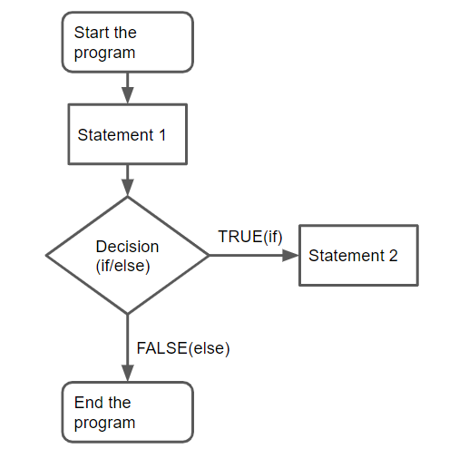
This definition can be illustrated by simple diagram shown below:

Knapsack Problem in DAA using Exhaustive Search

Given n items of known weights, w1, w2, …., wn and values v1, v2, …., vn and knapsack of capacity W, find the most valuable subset of the items that fit into the knapsack.

If you do not like the idea of putting yourself in the shoes of a thief who wants to steal the most valuable loot that fits into his knapsack, think about the transport plane that has to deliver the most valuable set of items to a remote location without exceeding the plane’s capacity.

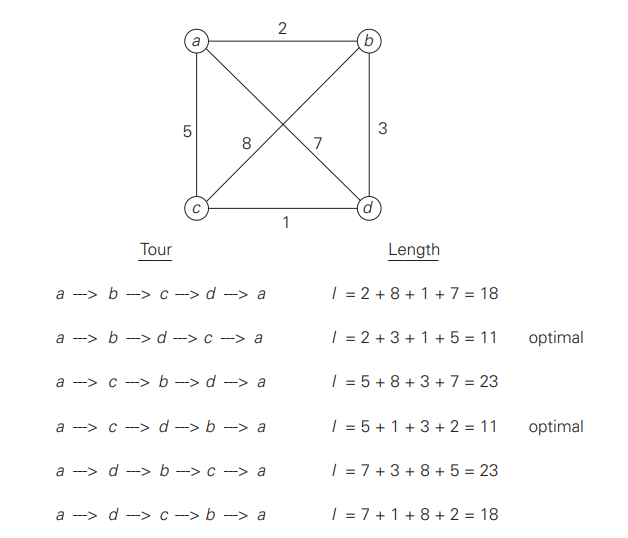
The exhaustive search approach to this problem leads to generating all the subsets of the set of n items given, computing the total weight of each subset in order to identify feasible subsets (ie., The ones with the total weight not exceeding the knapsack capacity), and finding the largest subset value among them.

The number of subjects of an element set is 2n, the exhaustive search leads to a Ω(2n) algorithm, no matter how efficiently individual subsets are generated.

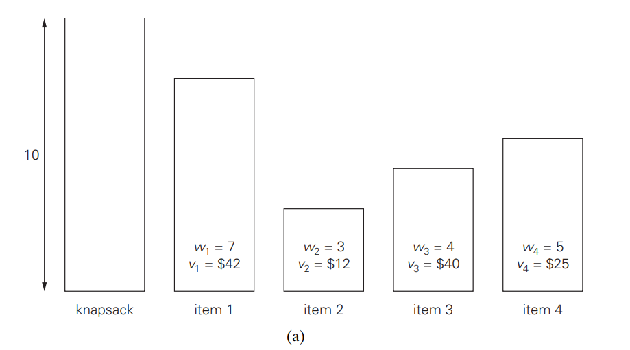
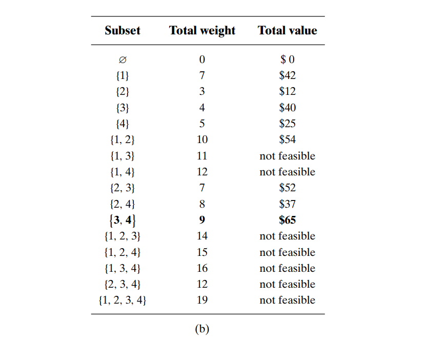
Figure: (a) Instance of the knapsack problem. (b) Its solution by exhaustive search.

The information about the optimal selection is in bold.

Thus, the knapsack problem considered above, exhaustive search leads to algorithms that are extremely inefficient on every input.
In fact, these two problems are the best-known examples of so-called NP-hard problems.
No polynomial-time algorithm is known for any NP hard problem.

0/1 Knapsack Problem using Branch and Bound

Let us now discuss how we can apply the branch-and-bound technique to solving the knapsack problem. Given n items of known weights wi and values vi, i = 1, 2, . . . , n, and a knapsack of capacity W, find the most valuable subset of the items that fit in the knapsack. It is convenient to order the items of a given instance in descending order by their value-to-weight ratios.

Then the first item gives the best payoff per weight unit and the last one gives the worst payoff per weight unit, with ties resolved arbitrarily:

v1/w1 ≥ v2/w2 ≥ ... ≥ vn/wn — (1)

Each node on the ith level of this tree, 0 ≤ i ≤ n, represents all the subsets of n items that include a particular selection made from the first i ordered items.

This particular selection is uniquely determined by the path from the root to the node.
A branch going to the left indicates the inclusion of the next item, and a branch going to the right indicates its exclusion.
A simple way to compute the upper bound (ub) is to add to v, the total value of the items already selected, the product of the remaining capacity of the knapsack W − w and the best per unit payoff among the remaining items, which is vi+1/wi+1:

ub = v + (W − w)(vi+1/wi+1) — (2)

Note:
As a specific example, let us apply the branch-and-bound algorithm to the same instance of the knapsack problem we solved above by exhaustive search.

Step-by-Step Explanation with Pseudocode

Branch and bound is used to solve the 0/1 knapsack problem efficiently by systematically exploring decision trees. Here’s a breakdown:

Initialization: Start with the root node representing no items selected and calculate its bound.
Priority Queue: Use a max-heap or priority queue to explore nodes based on their bound value.
Node Expansion: For each node:
- Generate child nodes by including or excluding an item.
- Calculate their bounds and prune infeasible nodes.
Termination: Stop when all nodes are processed or the queue is empty.

				
					function branch_and_bound_knapsack(items, capacity):
    initialize priority_queue
    root = create_root_node()  # no items, bound calculated
    priority_queue.push(root)
    max_profit = 0
    
    while priority_queue is not empty:
        current_node = priority_queue.pop()
        if current_node.bound > max_profit:
            for each child_node in expand(current_node):
                if is_promising(child_node):
                    if child_node.is_complete_solution():
                        max_profit = max(max_profit, child_node.profit)
                    else:
                        priority_queue.push(child_node)
    return max_profit

Let us now solve a Problem:

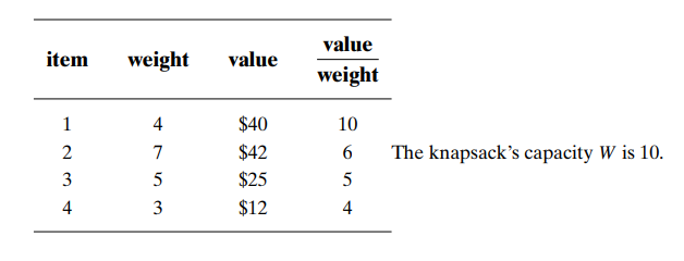
At the root of the state-space tree no items have been selected as yet. Hence, both the total weight of the items already selected w and their total value v are equal to 0. The value of the upper bound computed by formula (2) is $100.

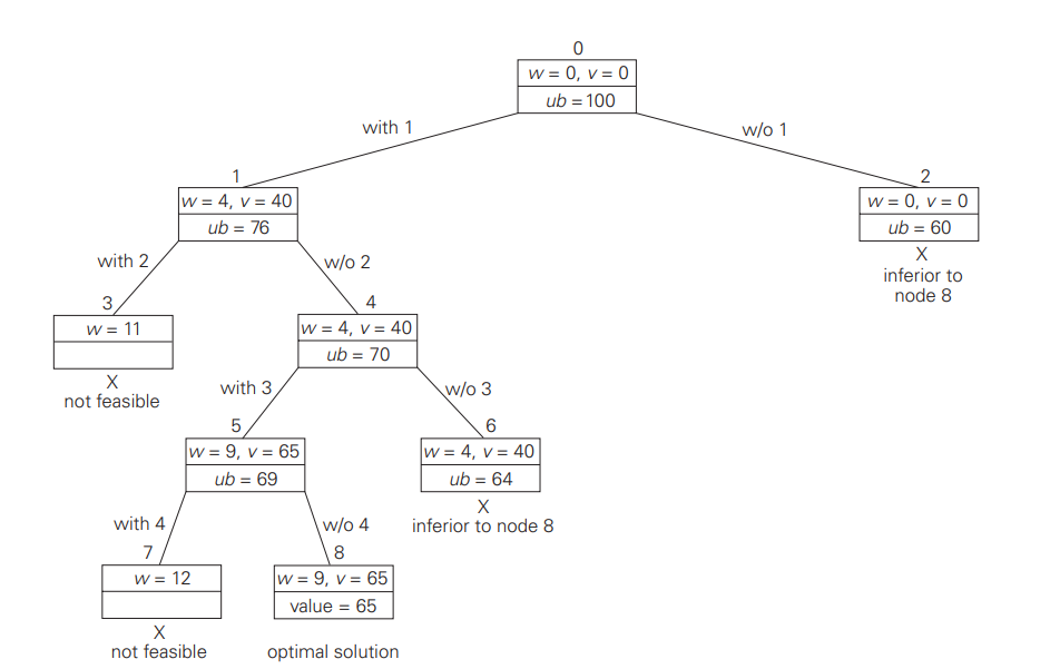
The above picture displays the State-space tree of the best-first branch-and-bound algorithm for the instance of the knapsack problem.

Node 1, the left child of the root, represents the subsets that include item 1.
The total weight and value of the items already included are 4 and $40, respectively; the value of the upper bound is 40 + (10 − 4) ∗ 6 = $76.
Node 2 represents the subsets that do not include item 1.
Accordingly, w = 0, v = $0, and ub =0+ (10 − 0) ∗ 6 = $60. Since node 1 has a larger upper bound than the upper bound of node 2, it is more promising for this maximization problem, and we branch from node 1 first.
Its children – nodes 3 and 4, represent subsets with item 1 and with and without item 2, respectively.
Since the total weight w of every subset represented by node 3 exceeds the knapsack’s capacity, node 3 can be terminated immediately.

Knapsack Visualization Tool

Enter Items as Weight, Value Pairs (e.g., 10,60 20,100):

Enter Knapsack Capacity:

Knapsack Problem Implementation using Java

				
					import java.util.Arrays;
import java.util.Comparator;
import java.util.PriorityQueue;

class Item {
	float weight;
	int value;

	Item(float weight, int value) {
		this.weight = weight;
		this.value = value;
	}
}

class Node {
	int level, profit, bound;
	float weight;

	Node(int level, int profit, float weight) {
		this.level = level;
		this.profit = profit;
		this.weight = weight;
	}
}

public class KnapsackBranchAndBound {
	static Comparator<Item> itemComparator = (a, b) -> {
		double ratio1 = (double) a.value / a.weight;
		double ratio2 = (double) b.value / b.weight;
		// Sorting in decreasing order of value per unit weight
		return Double.compare(ratio2, ratio1);
	};

	static int bound(Node u, int n, int W, Item[] arr) {
		if (u.weight >= W)
			return 0;

		int profitBound = u.profit;
		int j = u.level + 1;
		float totalWeight = u.weight;

		while (j < n && totalWeight + arr[j].weight <= W) {
			totalWeight += arr[j].weight;
			profitBound += arr[j].value;
			j++;
		}

		if (j < n)
			profitBound += (int) ((W - totalWeight) * arr[j].value / arr[j].weight);

		return profitBound;
	}

	static int knapsack(int W, Item[] arr, int n) {
		Arrays.sort(arr, itemComparator);
		PriorityQueue<Node> priorityQueue =
		new PriorityQueue<>((a, b) -> Integer.compare(b.bound, a.bound));
		Node u, v;

		u = new Node(-1, 0, 0);
		priorityQueue.offer(u);

		int maxProfit = 0;

		while (!priorityQueue.isEmpty()) {
			u = priorityQueue.poll();

			if (u.level == -1)
				v = new Node(0, 0, 0);
			else if (u.level == n - 1)
				continue;
			else
				v = new Node(u.level + 1, u.profit, u.weight);

			v.weight += arr[v.level].weight;
			v.profit += arr[v.level].value;

			if (v.weight <= W && v.profit > maxProfit)
				maxProfit = v.profit;

			v.bound = bound(v, n, W, arr);

			if (v.bound > maxProfit)
				priorityQueue.offer(v);

			v = new Node(u.level + 1, u.profit, u.weight);
			v.bound = bound(v, n, W, arr);

			if (v.bound > maxProfit)
				priorityQueue.offer(v);
		}

		return maxProfit;
	}

	public static void main(String[] args) {
		int W = 10;
		Item[] arr = {
			new Item(2, 40),
			new Item(3.14f, 50),
			new Item(1.98f, 100),
			new Item(5, 95),
			new Item(3, 30)
		};
		int n = arr.length;

		int maxProfit = knapsack(W, arr, n);
		System.out.println("Maximum possible profit = " + maxProfit);
	}
}

Output

Maximum possible profit = 235

Bonus:
Code Overview with detailed Explanation

The code implements the 0/1 Knapsack problem using the branch and bound algorithm, an efficient approach for exploring the solution space while avoiding unnecessary calculations.

Item Class: Represents each item with a weight and value. These are inputs for the knapsack problem.
Node Class: Represents nodes in the decision tree. Each node has:
- level: The index of the current item being considered.
- profit: Total profit accumulated at this node.
- weight: Total weight accumulated.
- bound: Upper bound of the maximum profit achievable from this node onward.
Priority Queue: Used to implement a max-heap based on the bound value to prioritize nodes with the highest potential profit.

Main Function:

1. Input Initialization:

Items are initialized with weights and values.
Capacity W and the number of items n are defined.

2. Knapsack Solution:

Call the knapsack function with capacity, item array, and number of items.
Print the maximum possible profit.

Conclusion

Solving the 0/1 knapsack problem by a branch-and-bound algorithm has rather unusual characteristics. Typically, internal nodes of a state-space tree do not define a point of the problem’s search space, because some of the solution’s components remain undefined.

For the knapsack problem, however, every node of the tree represents a subset of the items given. We can use this fact to update the information about the best subset seen so far after generating each new node in the tree. If we had done this for the instance investigated above, we could have terminated nodes 2 and 6 before node 8 was generated because they both are inferior to the subset of value $65 of node 5.

Frequently Asked Questions

What is knapsack problem with example?

The goal of the knapsack problem is to fit a set of objects into a container that has a maximum capacity, using predetermined values and sizes (such as weights or volumes). You are unable to pack every item if their combined size is greater than the available space.

Is knapsack greedy?

The Greedy Method is an effective way to solve the fractional Knapsack problem, which requires you to arrange the items in accordance with their weight to value ratio. We can break items in a fractional knapsack in order to increase the total value of the knapsack.

What is knapsack and its types?

The Knapsack Problem is an optimization problem where the goal is to identify the best solution out of all the potential combinations. 0/1 Knapsack, Fractional Knapsack, and Unbounded Knapsack are the three categories of knapsack problems. We will go into detail about 0/1 Knapsack problem using branch and bound in this article.

What is the knapsack like problem?

An example of an integer programming (IP) application is a knapsack problem. In knapsack problems, there are a number of items and a container (“Knapsack”) with a fixed capacity (Integer). Every item has a value (an additional integer) and a weight (an integer).